Project II - Portfolio optimization

We consider the problem of choosing a long term stock portfolio, given a set of stocks and their price over some period under risk aversion parameter γ > 0.

Assume there are m stocks to be considered. The portfolio will be represented by a column vector w ∈ ℝ^m, such that ∑_i=1..m w_i = 1. If w_i > 0, you use a fraction w_i of your total money to buy the i‘th stock, while w_i < 0 represent shorting that stock. In both cases we assume the stock is bought/shorted for the entire period.

Let p_j,i represent the price of the i‘th stock at time step j. If there are n + 1 time steps, then p ∈ ℝ^(n+1)×m is a matrix.

We let r ∈ ℝ^n×m be the matrix, where r_j,i represents the fractional reward of stock i at time step j, i.e., r_j,i = (p_j+1,i − p_j,i) / p_j,i for 1 ≤ j ≤ n.

By r_j we denote the j‘th row of r, viewed as a column vector (r_j,1, …, r_j,m).

We make the (unrealistic) assumption that we can model r by a random variable, distributed as a multivariate Gaussian, with estimated means

μ ≃ 1/n · ∑_j=1..n r_j

and estimated covariance matrix

Σ ≃ 1 / n · ∑_j=1..n [(r_j − μ)(r_j − μ)^T]

Note that μ_i and Σ_i,i are the estimated mean and variance for stock i.

The distribution of returns using some w is then

R_w = N(μ_w, σ_w²)

μ_w = w^Tμ

σ_w² = w^TΣw

Now, we want to maximize for a balance between high return μ_w and low risk σ_w². This leads to the following optimization problem, where we want to find the value w* of w maximizing the following expresion:

maximize     w^Tμ − γw^TΣw

subject to     ∑_i=1..m w_i = 1 ,

where γ controls the balance between risk and return. A high value of γ indicate we are willing to take low risk and vise versa.

In this project you should find w* for different values of γ and using real stock values of your choice. The project consists of the following three questions.

1. We need a module for collecting stock values, for this we will use the Python modyle yfinance that connects to Yahoo! Finance’s API. See https://pypi.org/project/yfinance/ for a description of how to install and use the module. Using this you should write a function get_prices([stocks, ... ], start, end, interval), that returns a tuple, (stocks, prices). Where prices[i, j] represent the opening price of stock j at time step i and stocks[j] is the name of the j‘th stock. Save the fetched data to a file, such that when requesting the same data again, the data is be loaded from the file instead of using the API (e.g., save a pandas dataframe as a csv file).

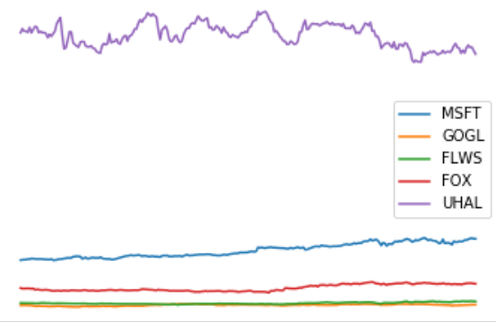
2. Plot the loaded price data. Each stock should be labeled with its name (for example MSFT or GOOGL). You should use at least 5 stocks. The legend should be ordered by the last price fetched for each stock. Plot both the raw stock prices and stocks normalized to all start with price 1.0.

3. Calculate r, μ and Σ using the formulas above and the prices p calculated in the first question. Plot the probability density function (pdf) of the return of each stock.
   Hint. The method norm.pdf from the module scipy.stats might become convenient. Note that it takes the mean and the standard deviation as arguments.

4. Solve the optimization problem defined above for different values of γ, e.g., gammas = numpy.linspace(1.0, 2.8, 10), and plot the pdf of each solution to a single plot with appropriate legends. Finally, create a scatter plot of how w* changes as γ changes. For each value of γ plot the fraction of each stock in the portfolio.